Analysis of matrix multiplications in transformer architectures

January 1, 2025

This analysis takes inspiration from Lequn Chen’s excellent article on transformer batching which analyzed performance on the A100 GPU. Building on their insights, this analysis focuses on the H100 architecture and provides fresh perspectives on transformer computations, with detailed performance analysis, comprehensive roofline model examination, and future optimization strategies specific to H100’s architecture.

Introduction

Transformer blocks are built on two primary types of matrix multiplications: dense layer operations and the QK multiplication in self-attention mechanisms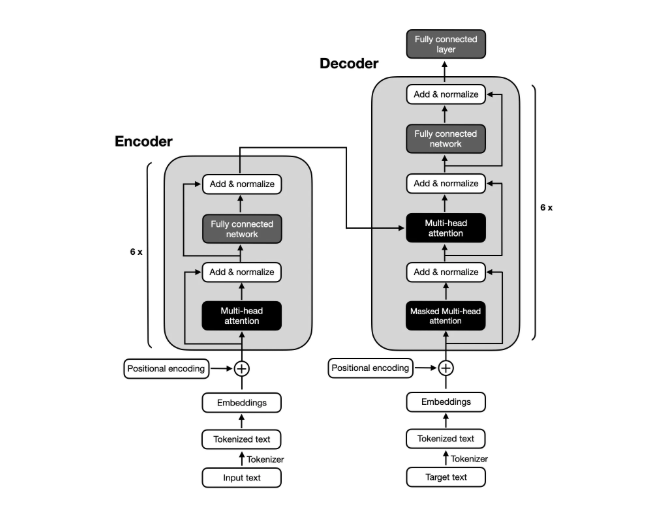

To understand more about the transformer block please read Sebastian Raschkas blogs. . These operations form the backbone of how Transformers process and encode input data, and their computational cost can be analyzed in terms of FLOPs (floating-point operations).

Dense Layers

Dense layers, are a fundamental component of Transformer blocks. These layers project inputs from one space to another. They are frequently used in the multi-head attention mechanism in projection operations, such as the generation of Q (query), K (key), and V (value) vectors in self-attention layers. Dense layers are also a crucial part of the Multi-Layer Perceptron (MLP) block, such as in models like LLaMA. A dense layer operates on an input tensor X of shape (batch,seqlen,h), where batch is the batch size, seqlen is the sequence length, and h is the hidden size. It uses a weight matrix W of shape (h,h) to perform a linear projection, producing an output tensor of the same shape (batch,seqlen,h)For higher-dimensional inputs, vector-matrix multiplication broadcasts across all dimensions except the last one. A dense layer of shape (h, h) applied to a tensor of shape (b, s, h) first reshapes to (b*s, h), performs the matrix multiplication, then reshapes back to (b, s, h).

Note: This broadcasting pattern is core to transformer architectures, allowing efficient parallel processing while preserving hidden dimension operations. through the matrix multiplication X⋅W.

Self Attention

The QK multiplication is a core operation in the self-attention mechanism of Transformer models, enabling the computation of how each token in a sequence “attends” to every other token. This operation generates the attention scores that underpin the model’s ability to contextualize the input. To begin, the input tensor X of shape (batch,seqlen,h), where batch is the batch size, seqlen is the sequence length, and h is the hidden size, is linearly projected into the Query (Q) and Key (K) matrices. Both Q and K have the same shape as X, (batch,seqlen,h), where h=n⋅d, with n being the number of attention heads and d the dimensionality of each head in Multi Head Attention.

FLOPs and IO

Dense Layer

The computational cost of this operation, measured in floating-point operations (FLOPs)Here FLOPs stands for number of floating point operations needed for the Matrix Multiplication, IO stands for number of Input and Output data transfer. In this current section these are not metrics of the Hardware(GPU). They are theoretical metrics. , is calculated as; each element in the output requires h multiplications and h−1 additions, approximately 2h operations per output element. With batch⋅seqlen⋅h output elements, the total number of operations is FLOPs = b⋅seqlen⋅h⋅(2h), which simplifies to

As a result, dense layers scale quadratically with the hidden size h, making them computationally expensive as h increasesThe computational complexity increases quadratically with the hidden size, making this a critical consideration for large models. .

The input matrix X has a shape of (b,seqlen,h), so the total number of elements read from X is b⋅seqlen⋅h. The weight matrix W, with a shape of (h,h), has h⋅h elements that are read. After performing the matrix multiplication X⋅W, the output matrix has the same shape as X, which is (b,seqlen,h), and the number of elements written to the output is b⋅seqlen⋅h.

Self Attention

Init

During initialization, when the entire sequence is processed at once, the Q and K matrices have the shapes (b, n, seqlen, d). To compute attention, the K matrix is transposed to (b, n, d, seqlen). The matrix multiplication Q⋅K^T then produces an output tensor of shape (b, n, seqlen, seqlen), where each element represents the attention score between a pair of tokens.

For each element in the output, d multiplications and (d−1) additions are required, totalling approximately 2d operations per element. Since the output matrix has seqlen⋅seqlen elements, and this computation occurs for each batch and head, the total number of FLOPs can be calculated as:

The Q matrix and K matrix have a shape of (b,n,seqlen,d), so the number of elements read is b⋅n⋅seqlen⋅d for both and the output attention scores have a shape of (b,n,seqlen,seqlen), so the number of elements written is b⋅n⋅seqlen^2. Adding all of them gives:

Auto-Regressive Step

In the auto-regressive phase, where tokens are processed incrementally, the computation is performed for only the current token against all previously decoded tokens. Here, the Q matrix has a shape of (b, n, 1, d), while the K matrix remains (b, n, seqlen, d). After transposition, K^T has the shape (b, n, d, seqlen). The resulting output tensor has the shape (b, n, 1, seqlen), representing attention scores for the current token against all preceding tokens.

For each output element, d multiplications and (d−1) additions are required, as before. However, since only seqlen elements are computed (instead of seqlen^2), the total FLOPs are:

The Q matrix has a shape of (b,n,1,d) so the number of elements read is b⋅n⋅1⋅d and K matrix has a shape of (b, n, seqlen, d), so the number of elements read is b⋅n⋅seqlen⋅d and the output attention scores have a shape of (b,n,1,seqlen), so the number of elements written is b⋅n⋅seqlen. Adding all of them gives:

Arithmetic Intensity

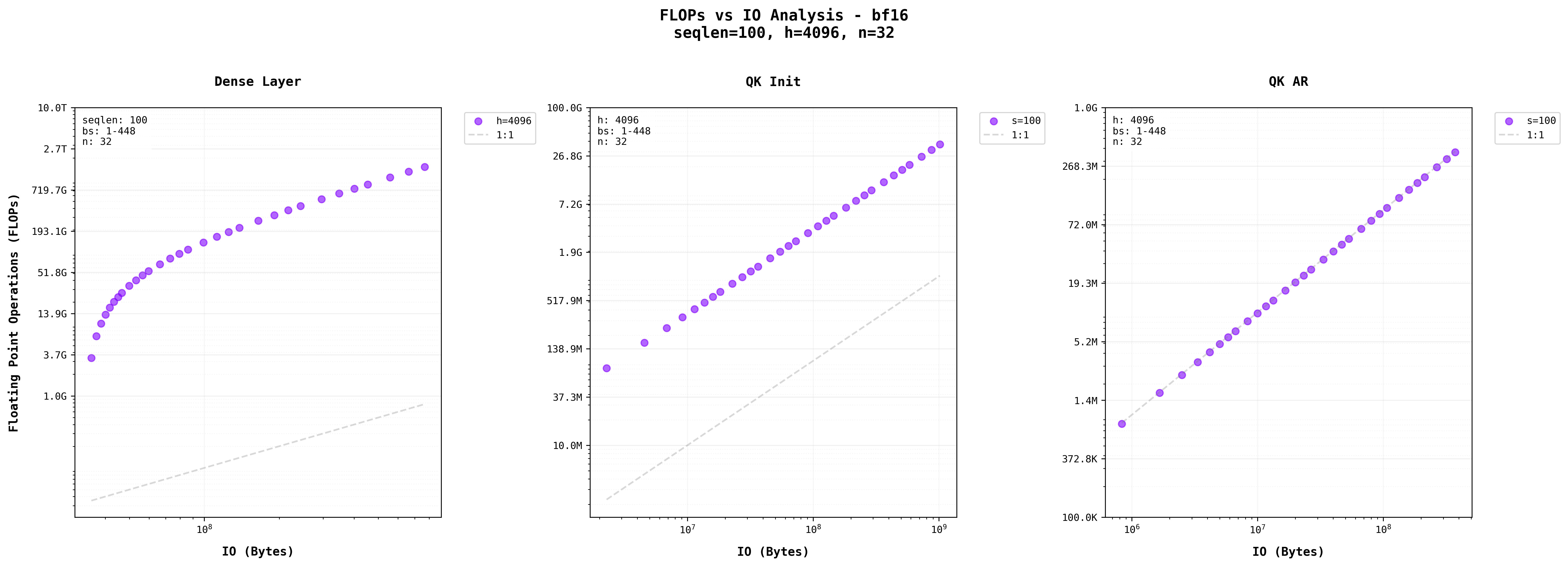
Arithmetic intensity is a critical metric that represents the ratio of computational operations (FLOPs) to memory operations (IO bytes), expressed as FLOPs/Byte

Arithmetic Intensity (AI) = FLOPs/Bytes is a key performance indicator that helps determine whether an operation is compute-bound or memory-bound. Higher AI values suggest compute-bound operations, while lower values indicate memory-bound operations.
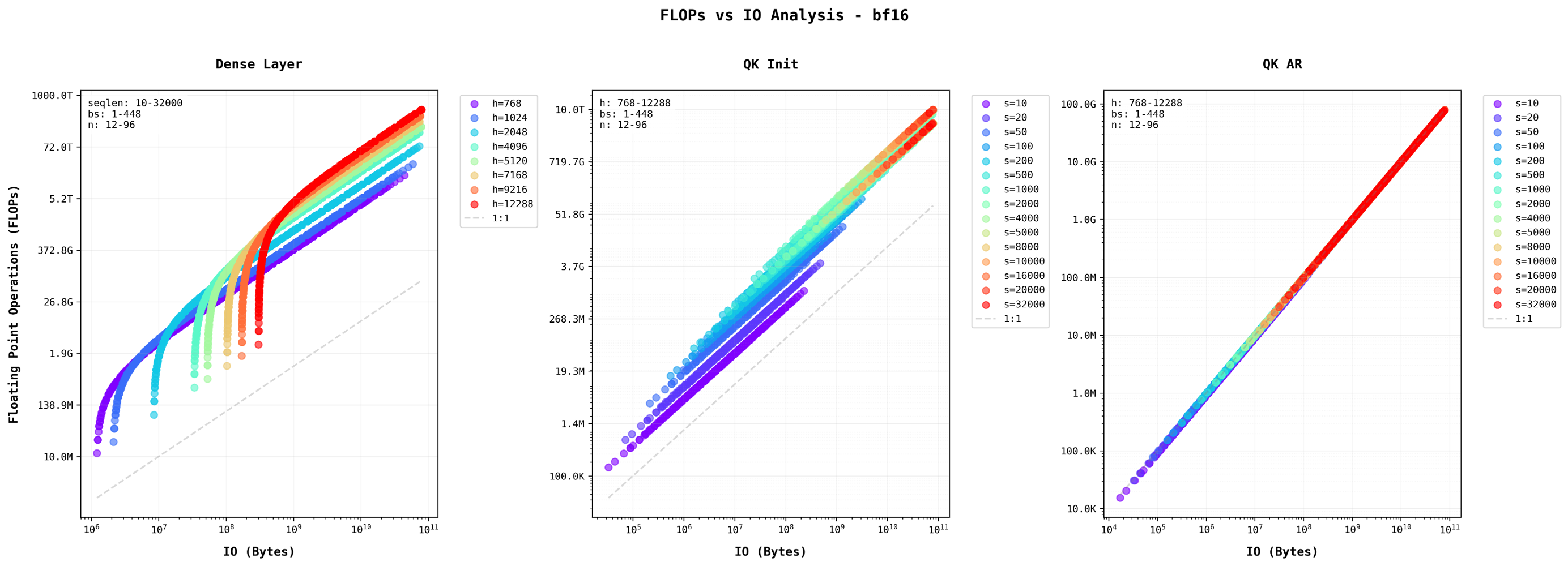
Read more here . The three plots visualize this relationship for different MatMul layers in Transformer blocks (Dense Layer, QK Init, and QK AR) using logarithmic scales on both axes, where each increment represents an order of magnitude increase. The diagonal gray line represents a 1:1 ratio between FLOPs and bytes, with points above this line indicating operations that perform more computations per byte of memory accessed.

For Dense Layers, the arithmetic intensity is governed by:

This results in quadratic scaling with hidden size (h), making these layers increasingly compute-intensive as models grow largerDense Layer Arithmetic Intensity:

\(\text{AI} = \frac{\text{FLOPs}}{\text{IO}} = \frac{2bsh^2}{2bsh + h^2} = \frac{2bsh}{2bs + h} = \frac{h}{1 + \frac{h}{2bs}} = O\left(\frac{1}{\frac{1}{h} + \frac{1}{2bs}}\right)\)

This ratio reveals key insights:
- When h is large: AI approaches O(b·s)
- As b·s increases: AI approaches O(h)
- When both h and b·s are large: AI is limited by min(h, b·s)

Note: Ive used s instead of seqlen for consistency with typical notation, but they represent the same sequence length parameter.

This mathematical relationship explains why increasing batch size improves efficiency: the denominator term 1/b approaches zero, maximizing arithmetic intensity. This is why dense layers in large models benefit significantly from batch processing. . The stepping pattern visible in the graph reflects this quadratic relationship, where larger hidden sizes show steeper curves and higher arithmetic intensity. This explains why dense layers in large models can become significant computational bottlenecks.

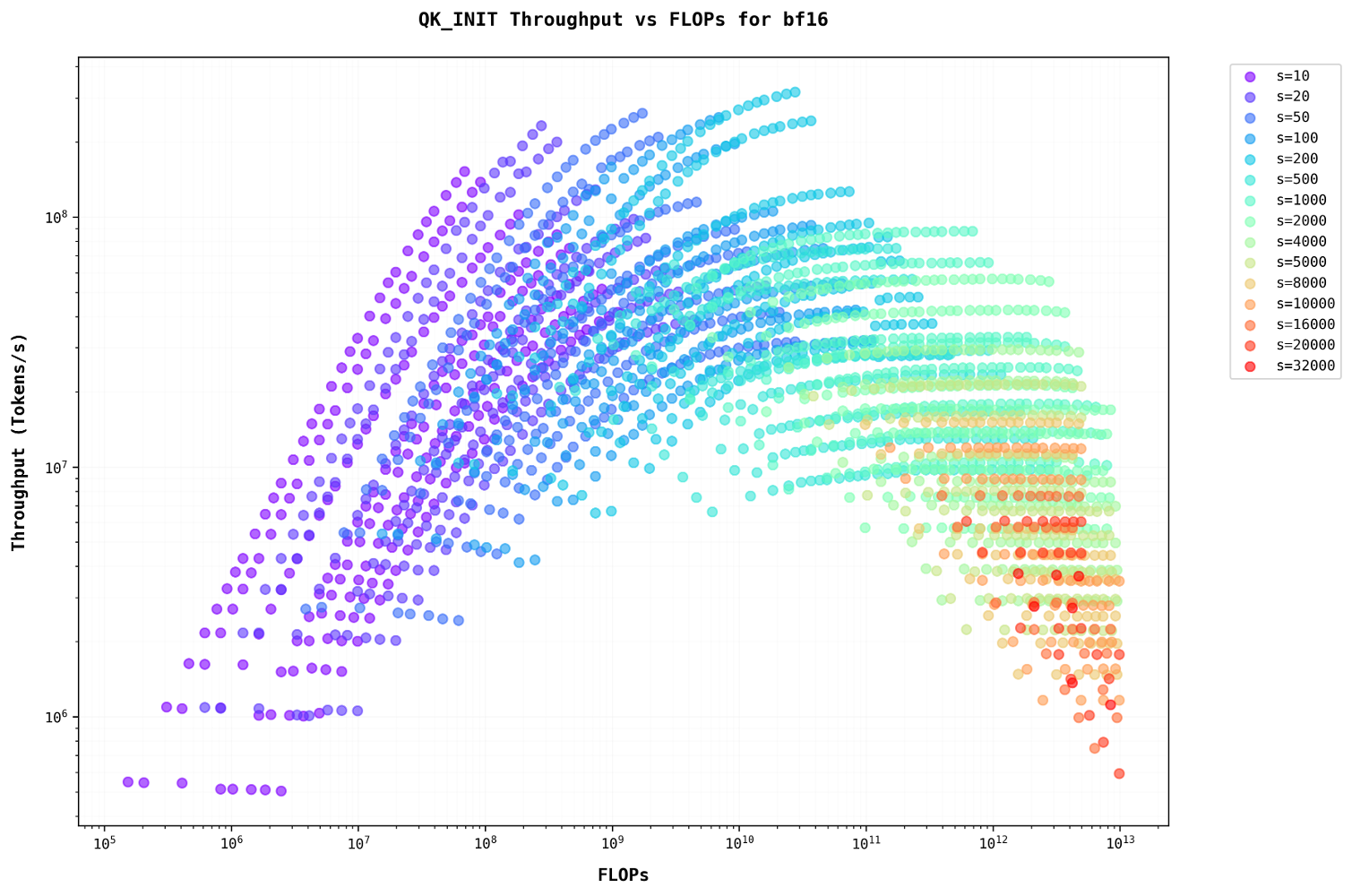
QK Init (Init) operations are characterized by:

The middle graph shows parallel lines for different sequence lengths, indicating consistent arithmetic intensity patterns that scale predictably with sequence length. So as the sequence length increases, they become more compute heavy thus higher seqlen in QK Init stage cause bottlenecks in the compute.

QK AR (Auto-Regressive) computations follow:

Unlike QK Init, this operation scales linearly with sequence length, resulting in more favorable arithmetic intensity characteristicsSelf-Attention Arithmetic Intensity:

For QK^T multiplication:
\(\text{FLOPs} = b \cdot n \cdot \text{seqlen}^2 \cdot 2 \cdot d\)
\(\text{IO} = 2(b \cdot n \cdot \text{seqlen} \cdot d) + (b \cdot n \cdot \text{seqlen}^2)\)

QK Arithmetic Intensity:
\(\text{AI} = \frac{\text{FLOPs}}{\text{IO}} = \frac{b \cdot n \cdot \text{seqlen}^2 \cdot 2d}{2bnd \cdot \text{seqlen} + bn \cdot \text{seqlen}^2} = \frac{2 \cdot \text{seqlen} \cdot d}{2d + \text{seqlen}}\)

This derivation reveals crucial properties:
- Batch size b cancels out completely
- AI depends only on sequence length and head dimension
- Scaling b increases both compute and memory linearly
- No inherent efficiency gain from batching unlike dense layers

The final expression shows why self-attentions performance characteristics remain constant regardless of batch size, making it fundamentally different from dense layer operations. . This is evident in the rightmost graph, where points cluster tightly along similar trajectories regardless of sequence length.

However, these graphs represent theoretical relationships that don’t account for real-world hardware constraints. The Roofline Model becomes crucial here as it helps bridge this gap by providing a framework to understand actual performance limitations. In the Roofline Model, performance is bounded by two primary factors: the peak computational performance (represented by a horizontal line) and the memory bandwidth limit (shown as a diagonal line). The lower of these two bounds at any given arithmetic intensity determines the maximum achievable performance. We’ll look at the roofline model in the sections below.

Analysis of Dense Layer

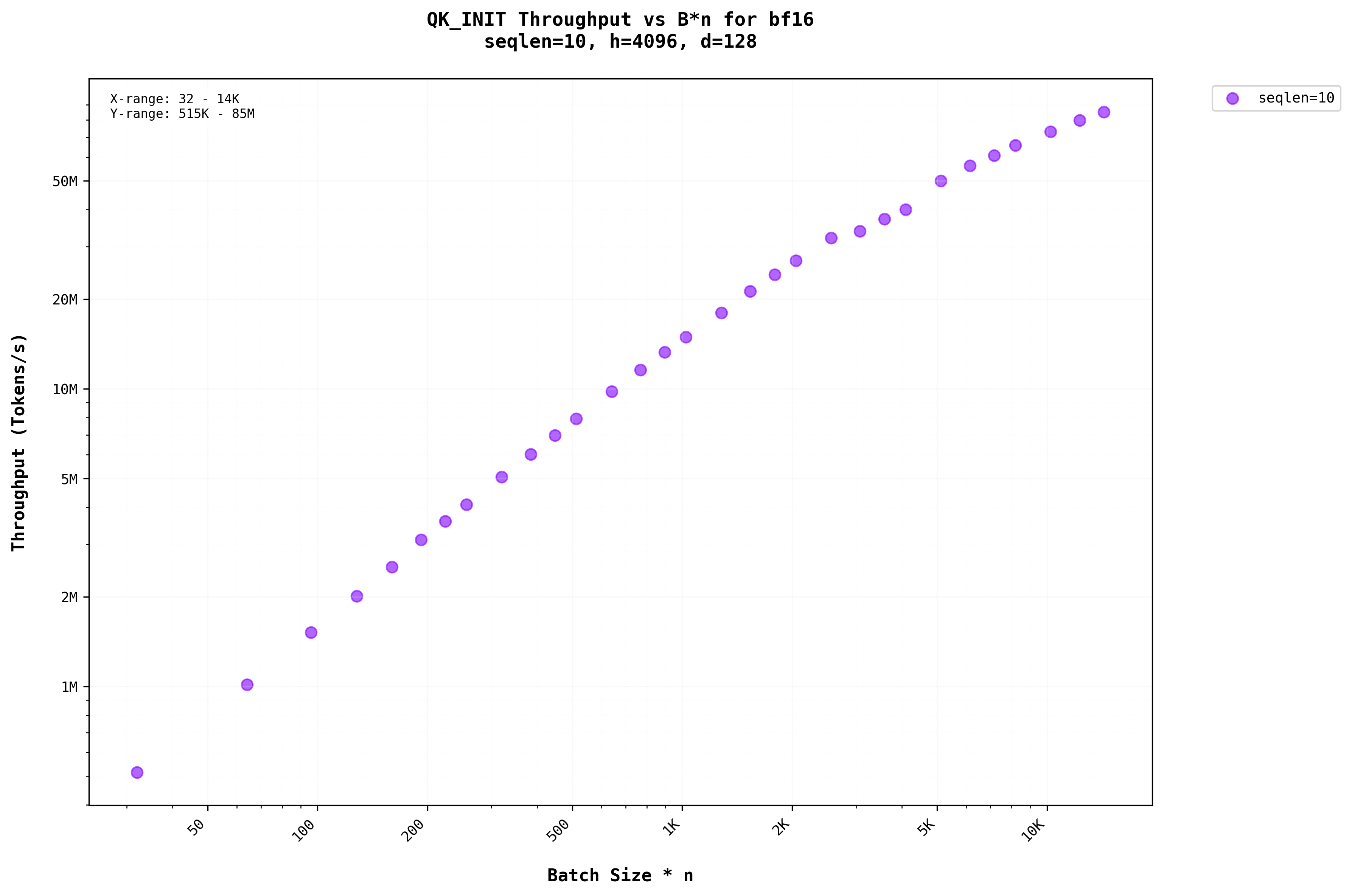
To analyze the dense layers, let’s look at the Throughput vs Batch graph. Throughput is calculated in tokens per second on the Y-axis and the X-axis shows the batch * seqlen dimension for that particular Dense operationFor higher-dimensional inputs, the vector-matrix multiplication is broadcasted to all dimensions except for the last one. For example, when applying a dense layer of shape (h, h) to a tensor of shape (b, s, h), the tensor is reshaped to (b*s, h) before the matrix multiplication and then reshaped back to (b, s, h) afterward. .

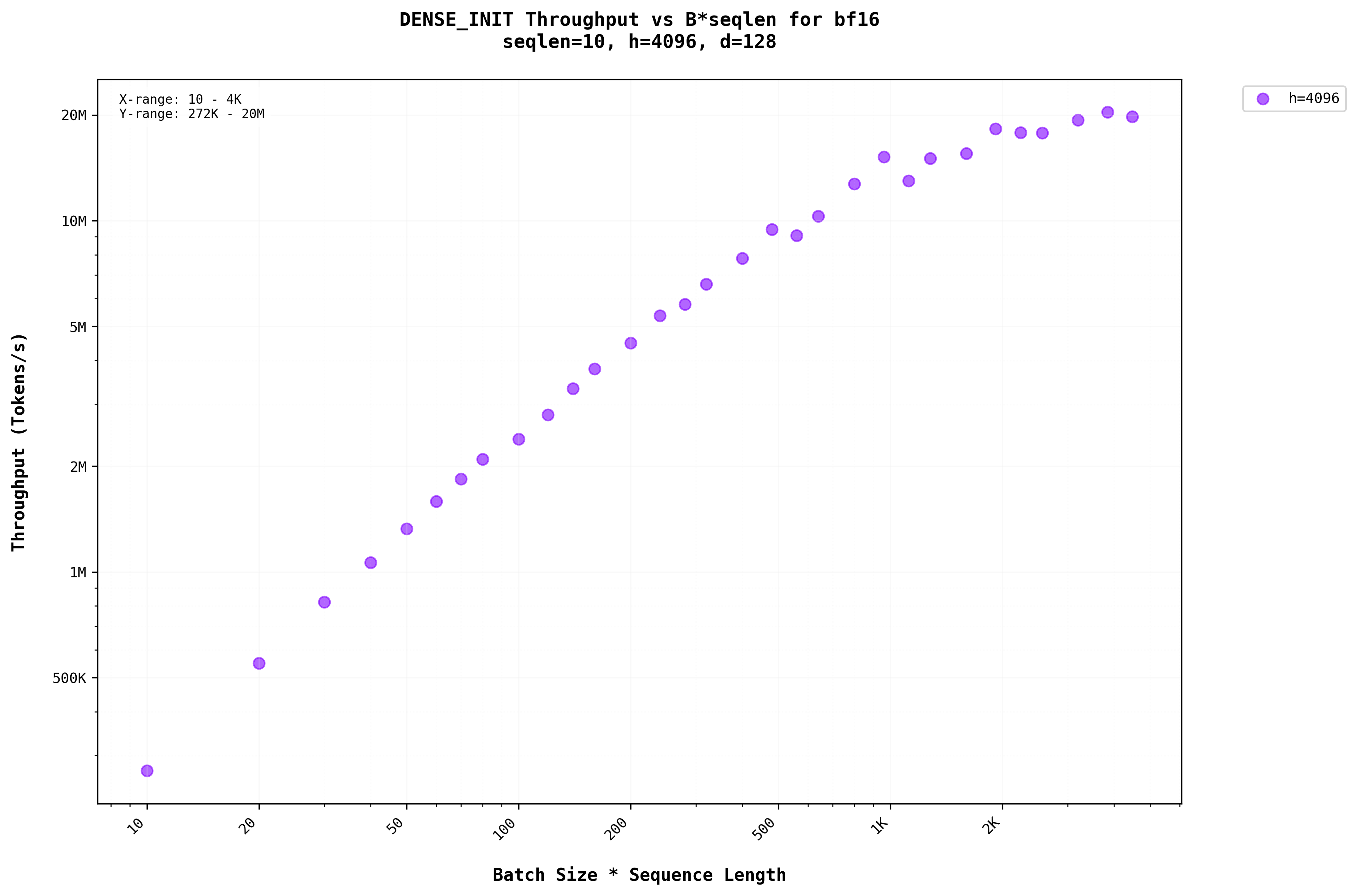
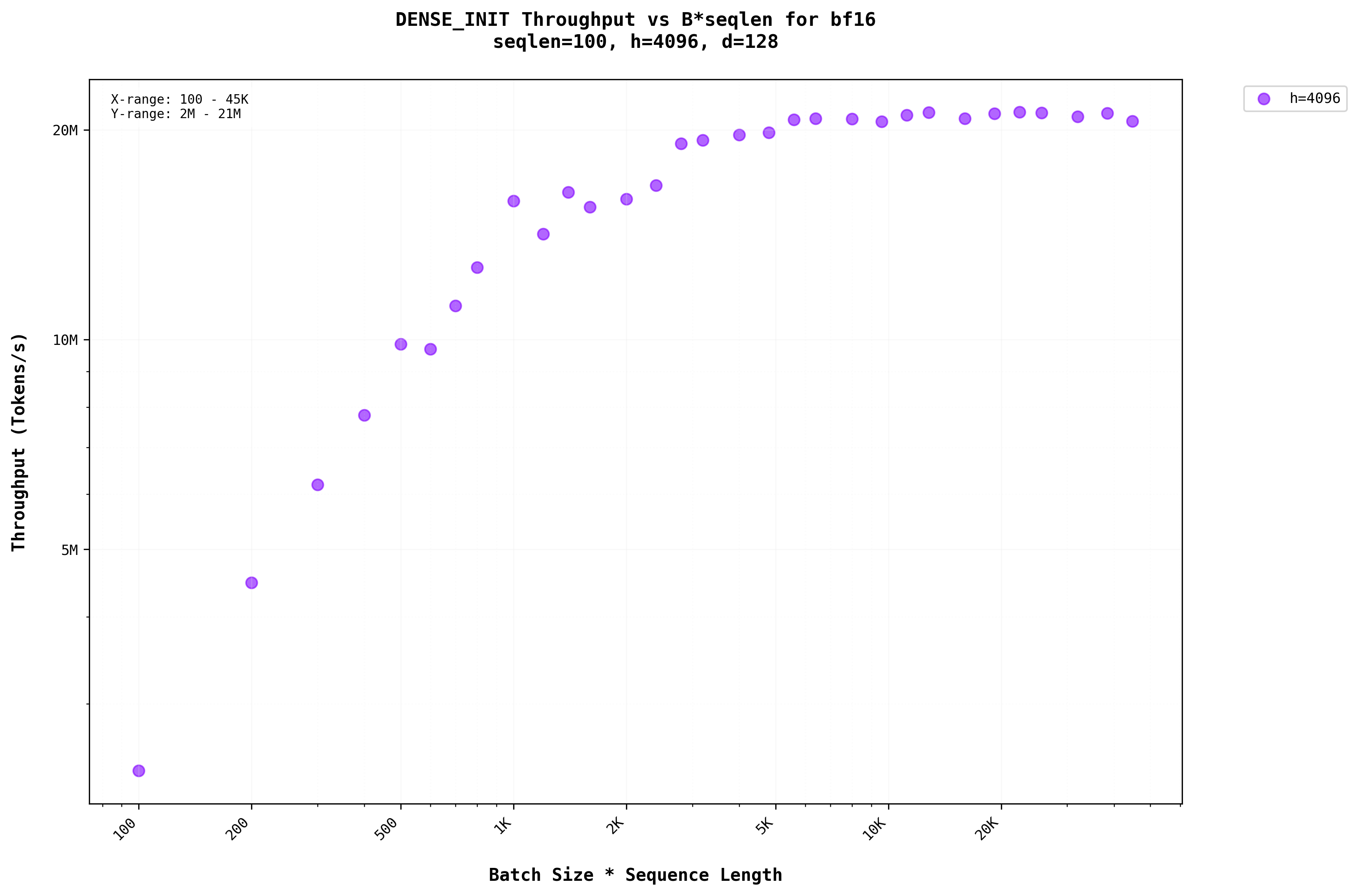
In Figure 3a, we can see that there is a benefit from batching. the throughput increases as the batch size increases. This is for the smaller dimension of the seqlen, but as the seqlen is made largerWhen the prompt is larger around 100+ tokens as the input , we can see that increasing the batch size improves the throughput only till a certain point but beyond that the throughput saturates as in Figure 3b.

We can infer that the H100 falls short of utilizing all the compute units for the matrix size when the input prompt is smaller but not for larger sequence lengths.

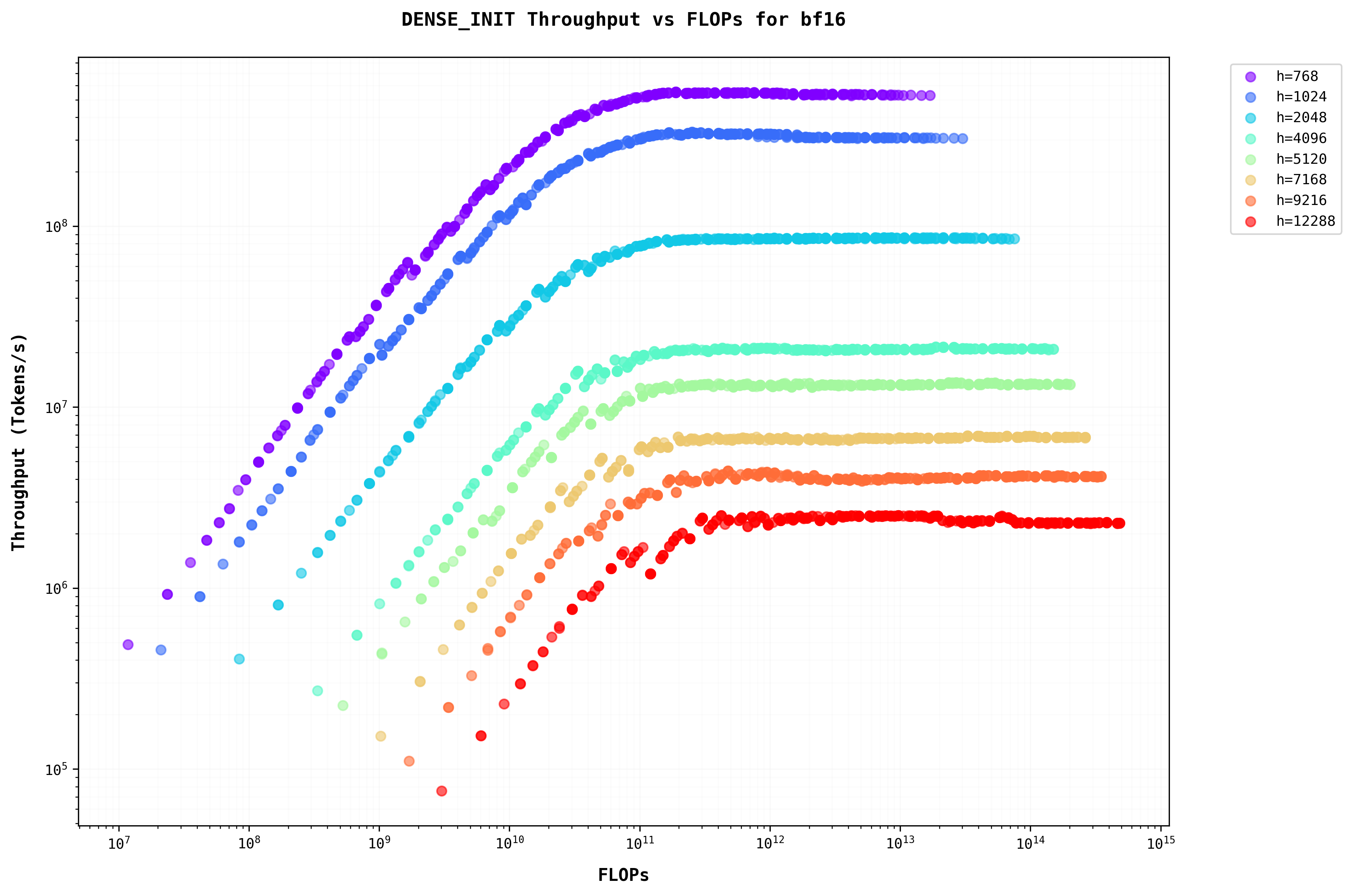
To show a consolidated view on Throughput vs the batch for all the batch dimensions with variations in h, d, n, and seqlen, it is not very useful to plot all of them separately for all the combinations of them. Instead using FLOPs on the x-axis allows us to analyze different model sizes on a single plot. This figure uses FLOPs as the x-axis, which is similar to b*s since FLOPs are O(bsh^2)The relationship between FLOPs and batch size demonstrates how computational complexity scales with model parameters, directly impacting throughput characteristics. . This plot shows that as the batch increases the also throughput increases when the seqlen is smaller (which is when the prompts are smaller). But if the batch is higher (either the batch is higher when the LLM is being served or the prompt is larger which causes seqlen to be larger or both) the throughput saturates.

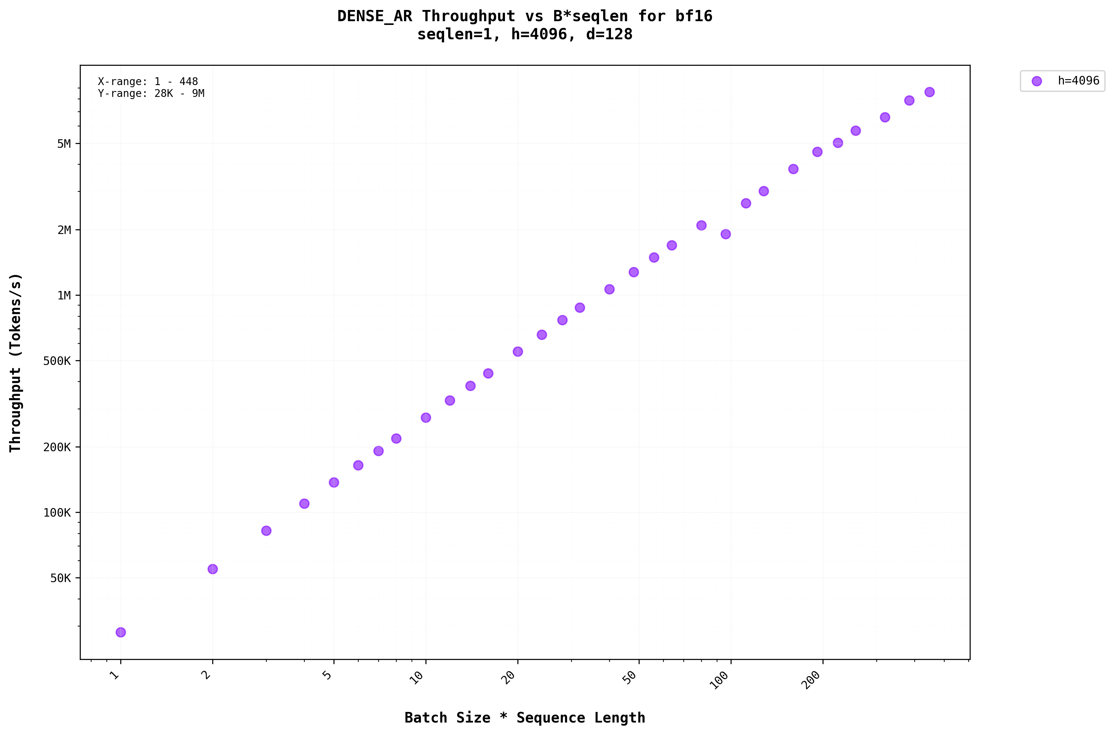
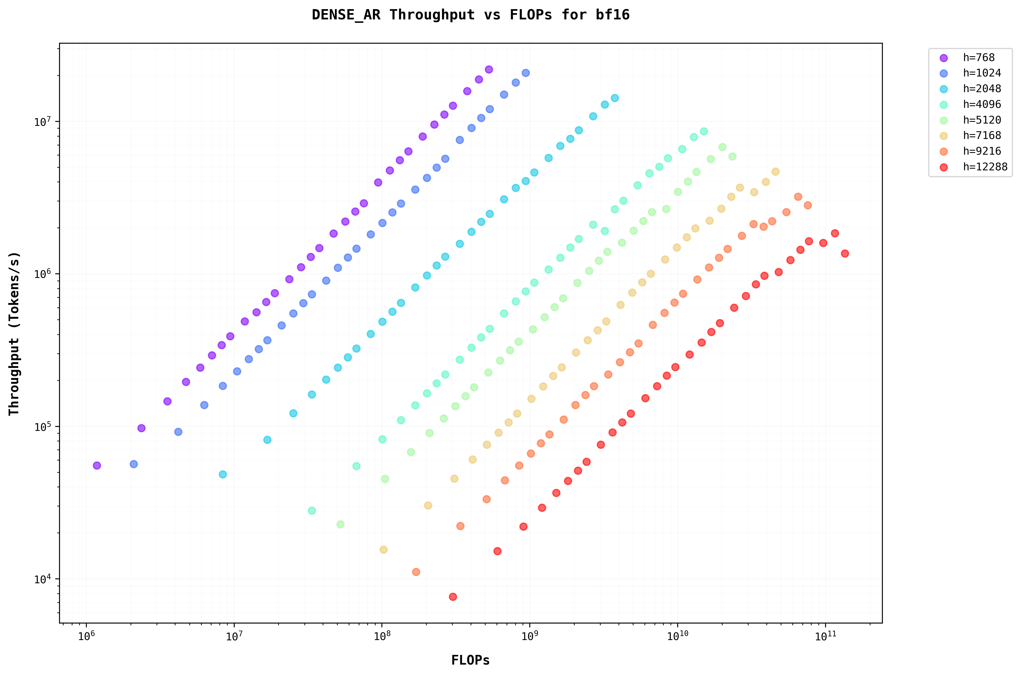
In the autoregressive(AR) stage, the sequence length is always 1The seqlen is 1 in AR step for dense because there is only the new Token which was generated in the previous step, that needs to be processed at this step. Keys and Values are needed for all the Tokens but this is handled by the KV Cache. Hence only 1 token processing gives us a seqlen = 1 . So there is no practical upper limit on the throughput even for higher batches. This reflects in the graphs from Figure 5a and 5b.

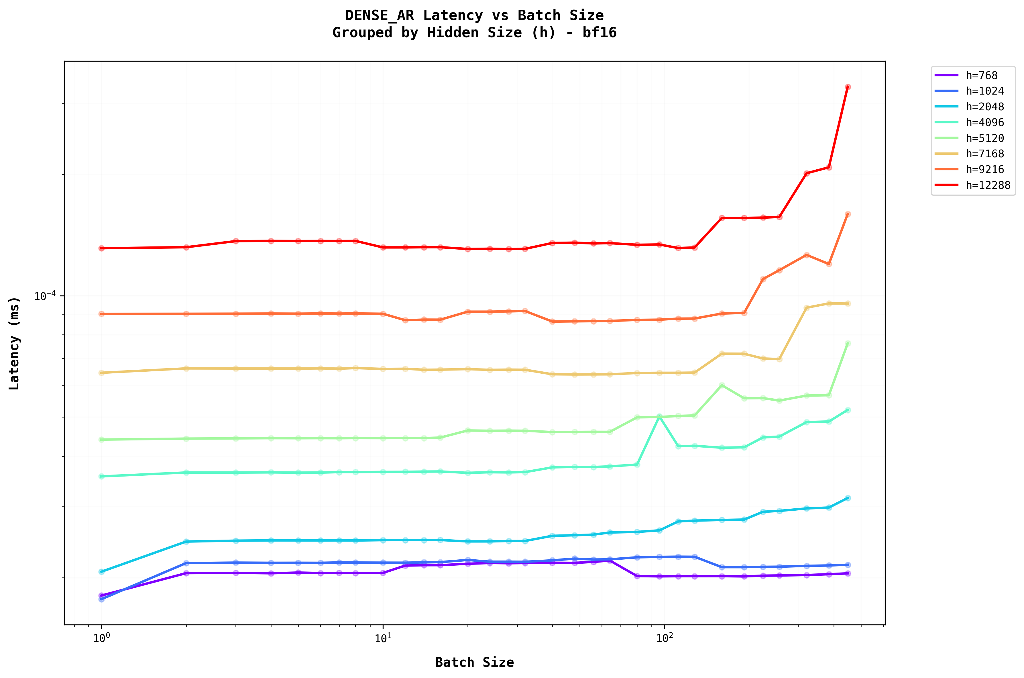
From Figure 6, we can see that batching dense layer in the auto regressive generation stage does not significantly affect the latency of the generation. This is a good thing because a batch of 100 has the same latency as that of lower batch sizes.

In system design, managing batch sizes and sequence lengths is crucial, particularly for larger models during the Init phaseThe relationship between batch size and sequence length creates a complex optimization space that directly impacts system performance and resource utilization. Understanding these dynamics is crucial for efficient model deployment. . This phase tends to be the primary performance bottleneck, requiring careful optimization to improve efficiency. Conversely, the autoregressive generation phase scales more effectively, making it less of a limiting factor in overall performance. Smaller models with hidden sizes below 2048 demonstrate better efficiency across both phases, highlighting their suitability for latency-sensitive applications. Additionally, effective batching strategies can significantly enhance the performance of the generation phase without incurring notable penalties. These insights suggest the need for distinct optimization strategies tailored to the Init and generation phases in model serving.

Analysis of Self Attention

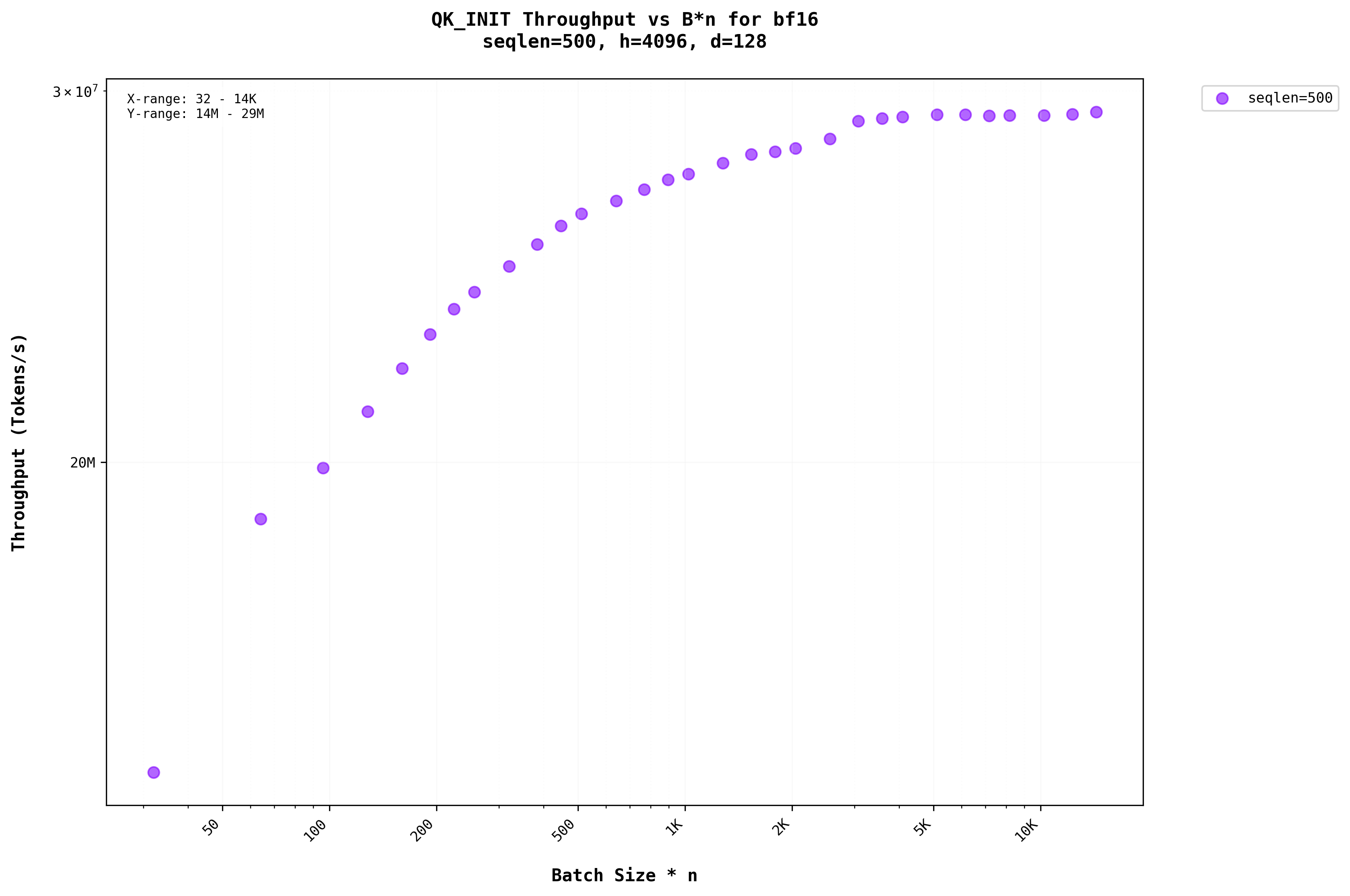
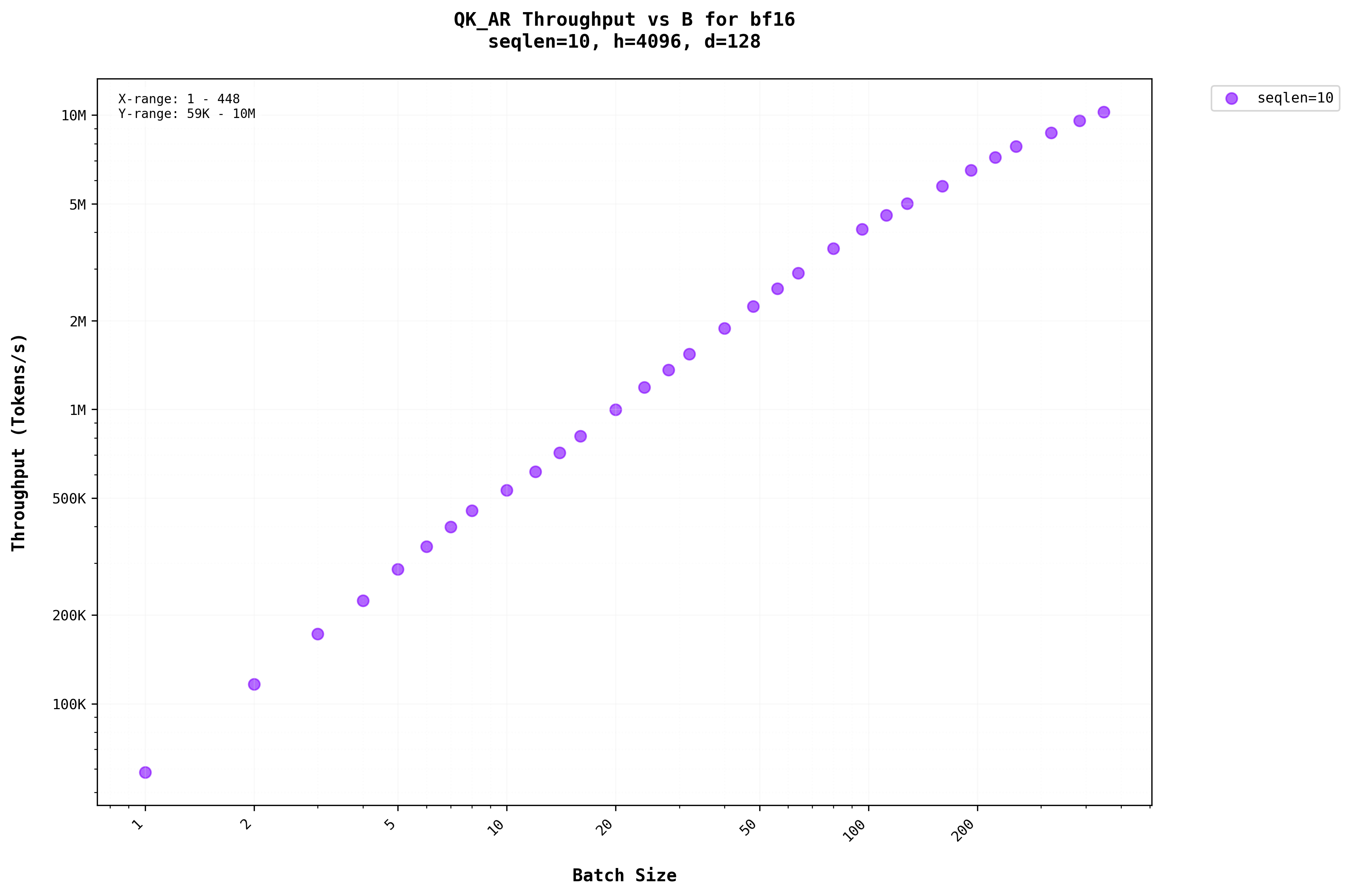
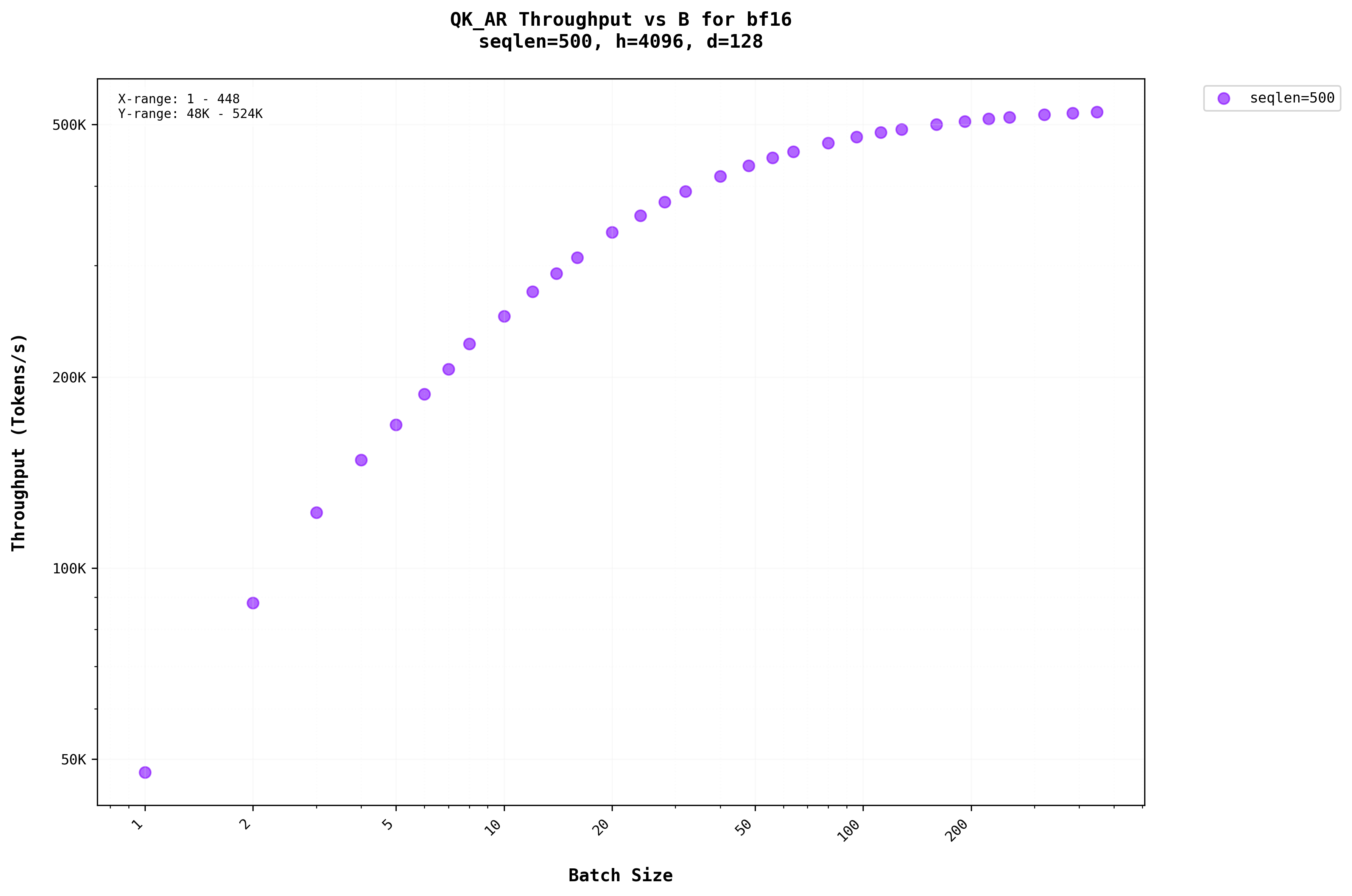
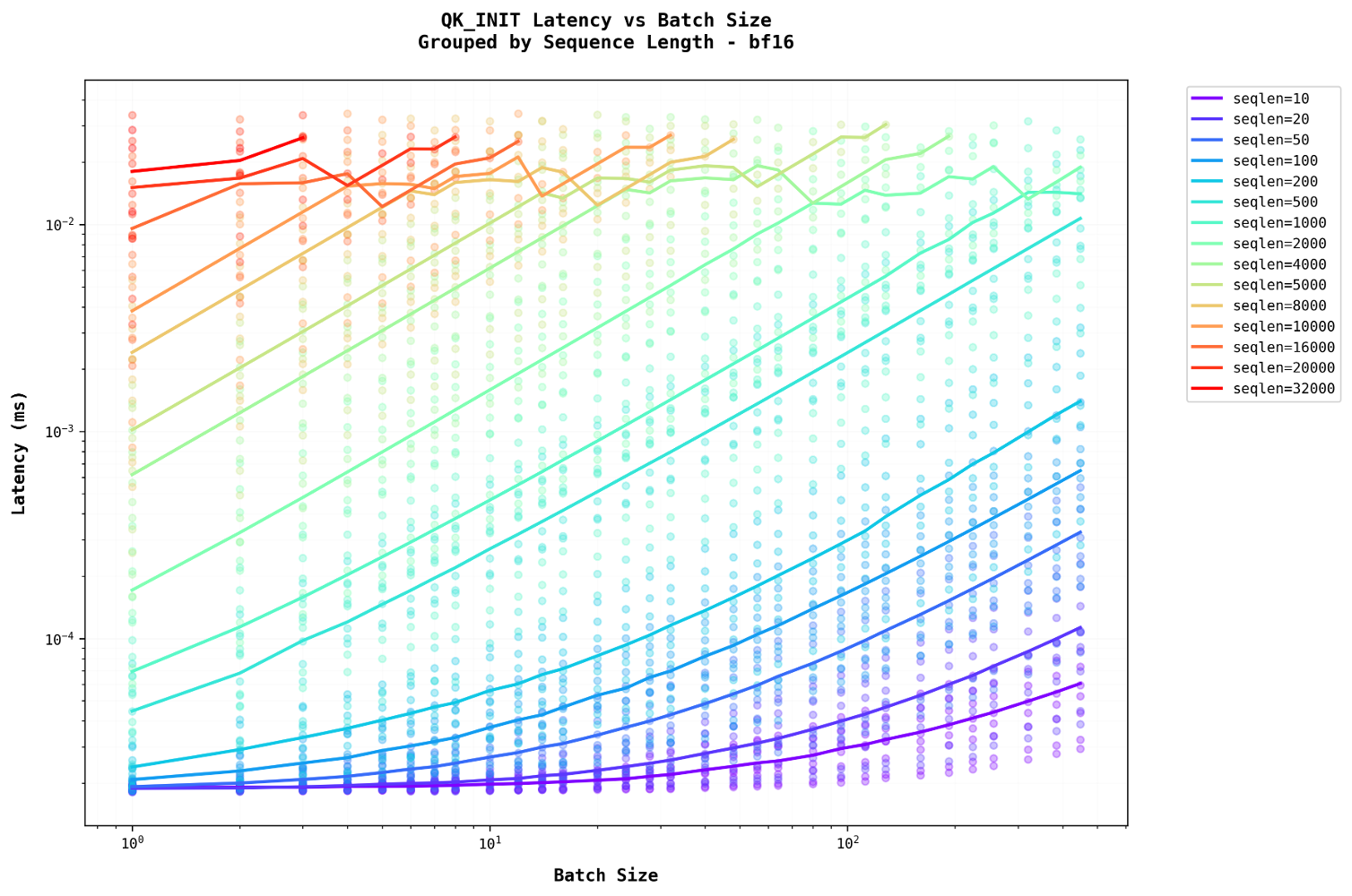
Analyzing the graphs above reveals that for smaller sequence lengths (shorter prompts) in the Init stage, batching has a more significant impact, providing noticeable benefitsThe impact of batching on self-attention performance varies significantly with sequence length, creating an important consideration for optimization strategies. . However, in the graph in Figure 7b, where the sequence length is larger (seqlen = 500) during the initialization stage, the throughput of the QK matrix multiplication begins to saturate as the batch size increases.

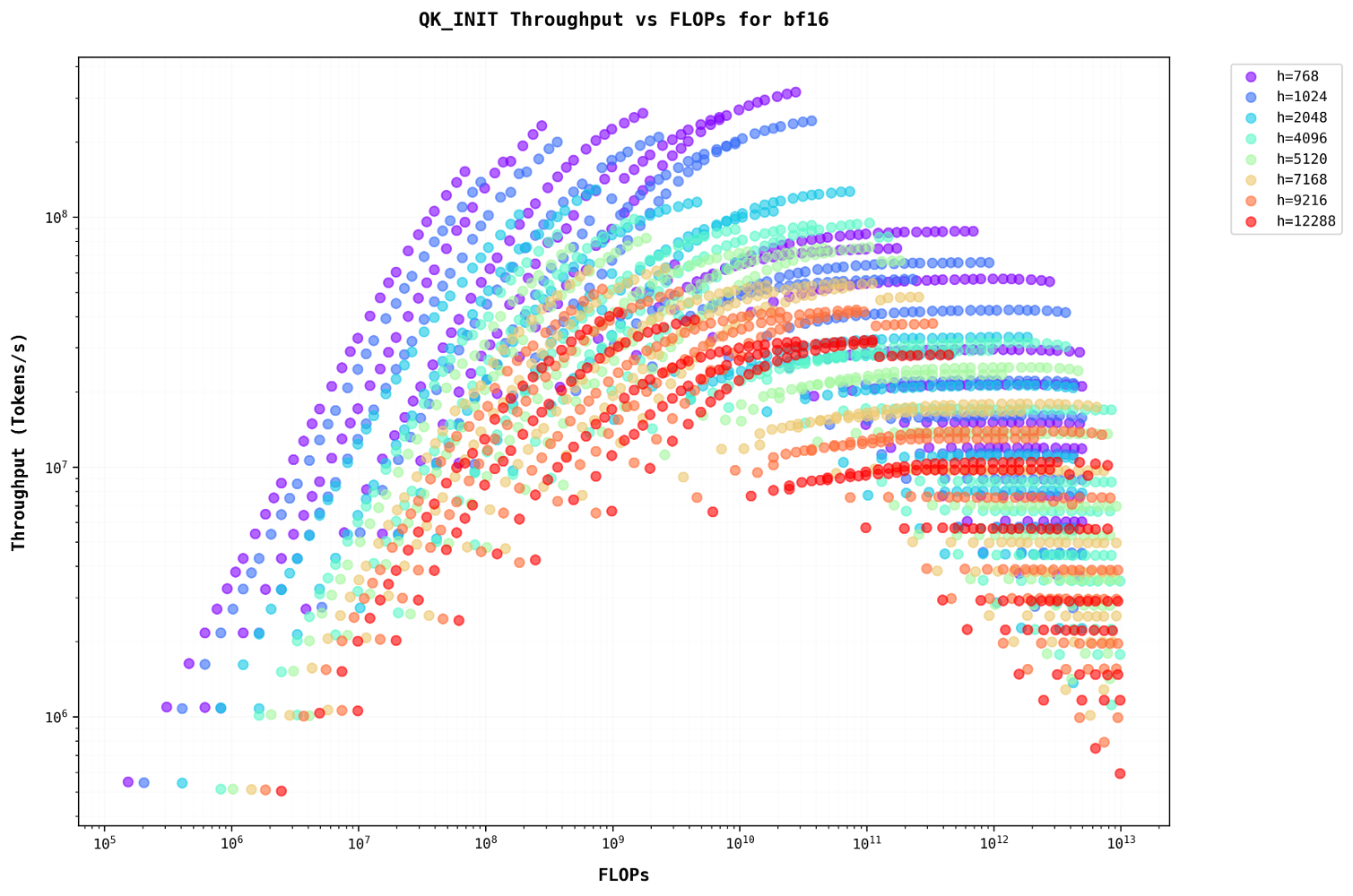
Let’s examine the plots with FLOPs on the x-axis, representing different model sizes on the same graphUsing FLOPs as a metric allows for direct comparison across different model configurations, providing insights into computational efficiency scaling. . For sequence lengths less than 500, throughput increases as the batch size grows. However, for sequence lengths greater than 500, the plots become linear, showing no increase in throughput despite an increase in batch size.

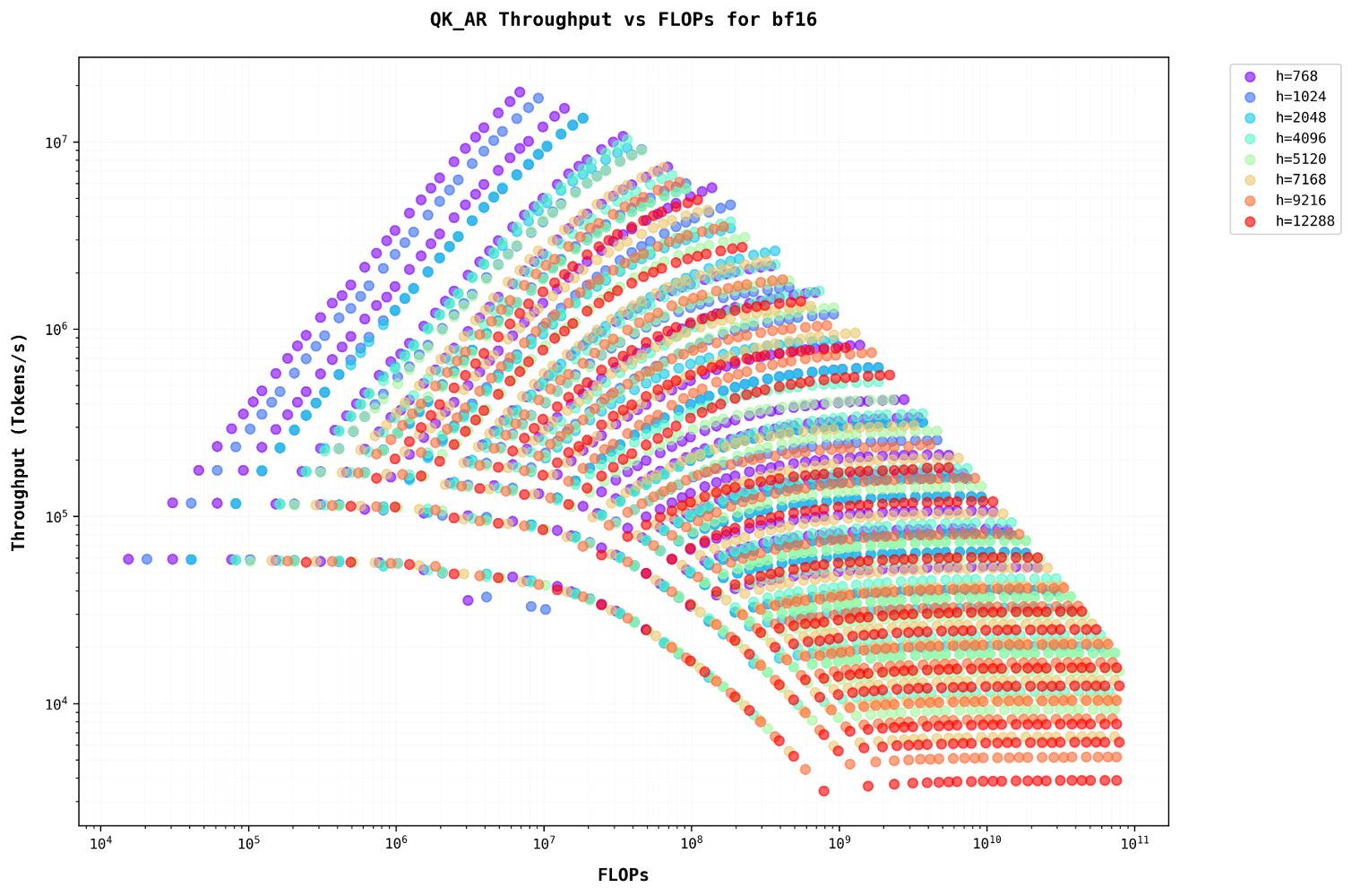
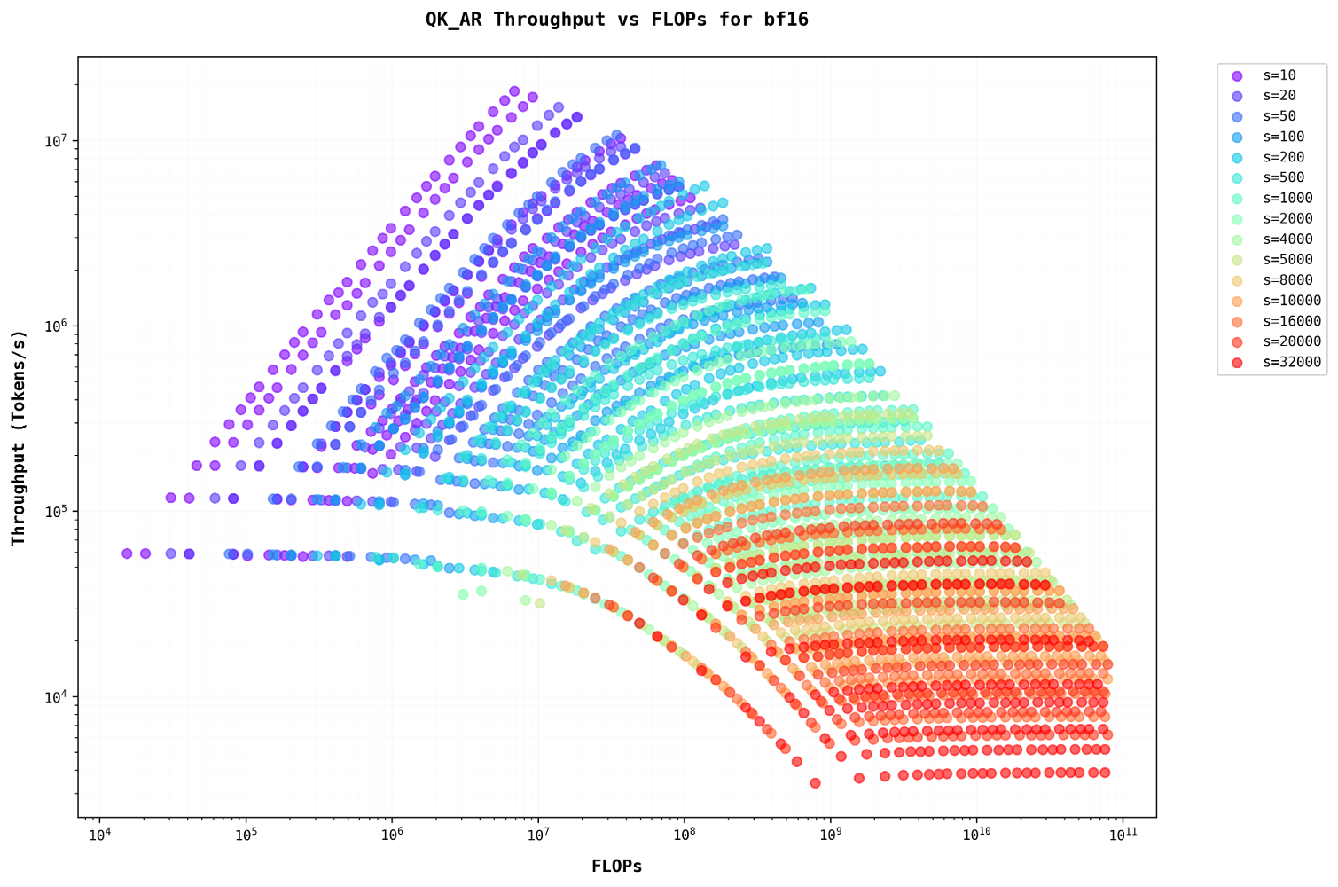
A similar pattern is observed in the auto-regressive stage, where increasing the batch size for larger sequence lengths has minimal to no effect. This occurs because they share a similar Arithmetic Intensity. Additionally, as auto-regression progresses, the sequence length increases, further diminishing the impact of batching.

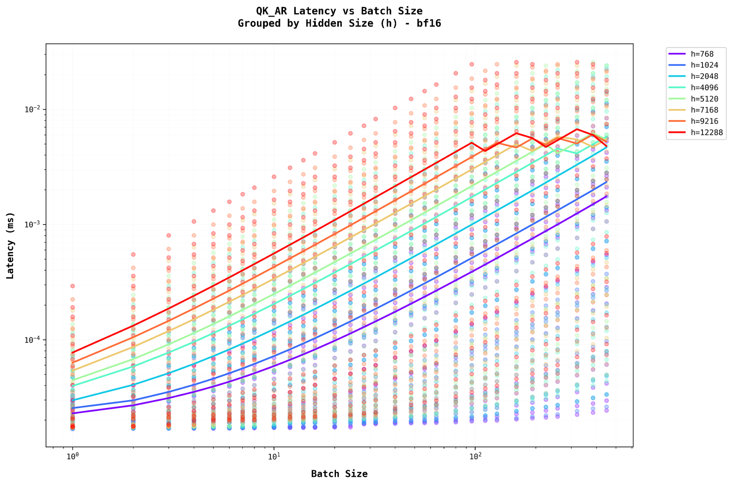
Self-attention latency is comparable to that of a dense layer but increases with batch size, unlike a dense layer. This latency scales approximately linearly with batch size because self-attention primarily involves batched matrix multiplication. With a fixed FLOP-to-I/O ratio, increasing the batch size proportionally raises both FLOPs and I/O, maintaining a constant ratioSelf-Attention Arithmetic Intensity:
\(\text{QK AI} = \frac{2 \cdot \text{seqlen} \cdot d}{2d + \text{seqlen}}\)

- Batch size b cancels out completely
- AI depends only on sequence length and head dimension

Therefore, increasing batch size does not change the AI, it increases both FLOPs and IO at the same multiplier. . For example, increasing the batch size from 100 to 1000 directs the system to process more items simultaneously, boosting total throughput without accelerating the processing of individual items. The fundamental matrix multiplication operations still require the same number of steps per item, as the computational work (FLOPs) and memory operations (I/O) scale together. Additionally, in auto-regressive tasks, as the sequence length grows, more time is required to process each subsequent step.

Roofline Model

The roofline model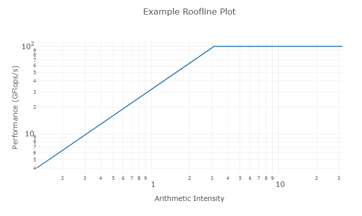

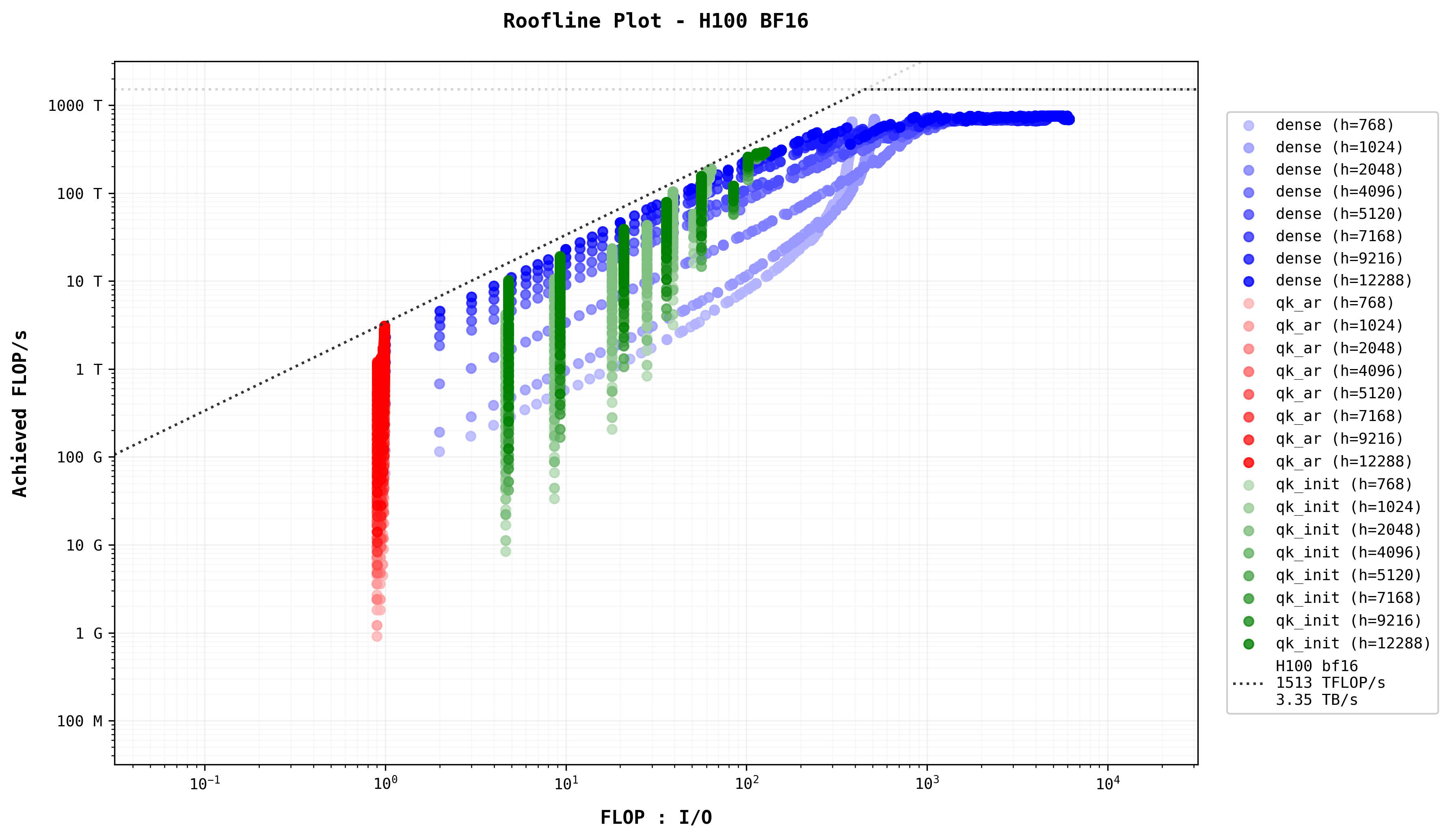
The Roofline Model is a performance model seeking to give the limitations of a specific hardware component in terms of algorithm performance. The model is often employed visually as a log-log plot of Arithmetic Intensity vs Flops/s. Read the math behind it here presents the data points for all benchmark combinations, organized using the Roofline Model. Different stages and layers are distinguished through color coding. Overlaid on the figure are the theoretical memory bandwidth and FLOP/s limits, based on NVIDIA H100 specifications.

Two key insights emerge from this visualization:

1. The data points cluster into distinct groups and sub-groups, naturally reflecting the computational and memory characteristics of various stages and layers.
2. The data points closely follow the theoretical roofline, demonstrating that the benchmarks effectively leverage the hardware’s capabilities relative to its peak performance.

To observe the impact of batching, let’s examine a specific case (h=4096, s=100)

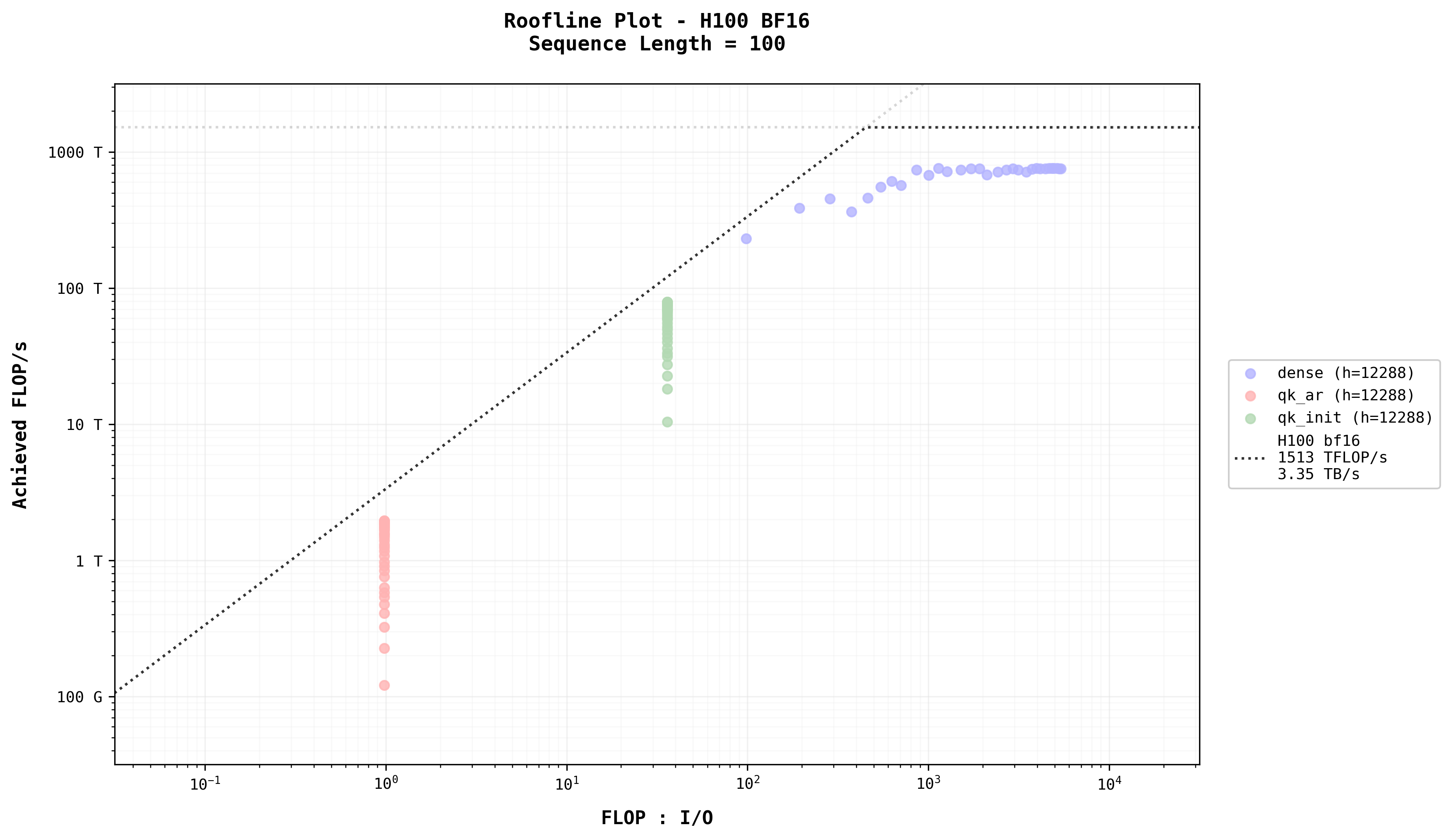
• Arithmetic Intensity and Achieved FLOP/s: Arithmetic intensity across operations follows the sequence: dense_init > qk_init > dense_ar > qk_ar. Achieved FLOP/s also follows this order. The dense layer during initialization is constrained by the GPU’s peak computational performance. For small models and short sequence lengths, batching provides slight improvements, but significant performance gains require investing in a more powerful GPU.
• Dense Layer in Auto-Regression: Unlike initialization, the dense layer in the auto-regression stage behaves differently. For the same model size, its data points align with the slope of the GPU’s memory bandwidth, indicating that its performance is memory bandwidth-bound. Under this constraint, increasing the batch size enhances the achieved FLOP/s by improving arithmetic intensity.
• Batching and Self-Attention: Batching significantly impacts self-attention. While it does not alter the arithmetic intensity of self-attention, it increases the achieved FLOP/s for short sequence lengths by enabling parallel processing.
• Kernel Implementation in Self-Attention: The increase in achieved FLOP/s for self-attention, despite unchanged arithmetic intensity, suggests that the kernel implementation may be suboptimal, potentially failing to fully utilize the GPU’s compute units.

Data Availability

All the data used in this analysis is publicly available in CSV format at transformer_bench/data. While this article focuses on bf16 dtype results, the repository contains data for fp32 and fp16 dtypes as well on the H100 GPU. You are encouraged to perform their own analysis using these additional precision formats and contribute their findings to the repository at doteval/transformer_bench.

Summary

• Performance Hierarchy and Hardware Constraints
  • Arithmetic intensity and achieved FLOP/s follow a clear hierarchy: dense_init > qk_init > dense_ar > qk_ar
  • Dense layer initialization is compute-bound by GPU peak performance
  • Dense layer auto-regression is memory bandwidth-bound
  • Performance improvements in compute-bound operations require GPU upgrades, while memory-bound operations benefit from optimized batching strategies
• Sequence Length and Batching Dynamics
  • Short sequence lengths (< 500 tokens) show significant benefits from batching
  • Longer sequences (> 500 tokens) show diminishing returns from increased batch sizes
  • In autoregressive generation, sequence length remains at 1, allowing for efficient batching
  • Throughput saturation occurs at different batch sizes depending on sequence length and model size
• Self-Attention Characteristics and Optimization
  • Self-attention benefits from batching without changing arithmetic intensity
  • Current kernel implementations show signs of suboptimal compute unit utilization
  • Parallel processing capabilities are not fully exploited, suggesting room for optimization
  • Performance scales linearly with batch size due to the nature of matrix multiplication operations
• Model Size Considerations
  • Smaller models (hidden sizes < 2048) demonstrate better efficiency across all phases
  • Larger models face significant computational bottlenecks during Init
  • Memory bandwidth becomes a limiting factor for large models in autoregressive phase
  • Different optimization strategies are needed for different model sizes
• System Design and Implementation Insights
  • Init phase is typically the primary performance bottleneck
  • Autoregressive generation phase shows more favorable scaling characteristics
  • Different phases require distinct optimization approaches due to varying performance characteristics
  • System designs need to balance between throughput optimization and latency requirements based on use case

Future

Optimizing Self-Attention Through Matrix Fusion

In the self-attention mechanism, we can identify a key optimization opportunity in the matrix multiplication operations. Currently, the computation flow involves:

1. Computing QK^T which produces an intermediate result with shape (b, n, s, s)
2. Applying softmax to this intermediate result
3. Multiplying with V to get the final output of shape (b, n, s, d)

A more efficient approach would combine these operations into a unified computation:

1. The key insight is that we can fuse these three matrix operations (QK^T, softmax, and multiplication with V) into a single GPU kernel operation
2. This fusion is particularly effective because the head dimension (d=128) is relatively small
3. The main challenge lies in handling the softmax operation, which traditionally requires computing across the entire sequence dimension

The softmax computation presents a specific challenge, but this was solved beautifully by Flash Attention. There are 3 versions of Flash Attention. 3rd being a specific optimisation to H100 GPUS, and the first 2 papers can be implemented in any GPU. Links to the papers are in the references.

Efficient Request Batching Strategy

Analysis revealed significant potential in batching multiple requests, even when they have different sequence lengths. Rather than using simple padding, we can implement a more sophisticated approach based on our performance analysis:

Key Observations:

1. Dense layer performance:
   • Shows strong batching benefits
   • Maintains nearly constant latency during autoregressive generation
   • Treats sequence dimension similarly to batch dimension
2. Self-attention characteristics:
   • Must process each sequence independently
   • Cannot be batched across different sequences
   • Takes less execution time compared to dense layers

Implementation Strategy:

1. Input Processing:
   • Take variable-length inputs: [(s1, h), (s2, h), ...]
   • Combine them into a single matrix: (sum(si), h)
2. Computation Flow:
   • Process the combined matrix through dense layers
   • Split the results back into individual sequences
   • Handle self-attention computations separately for each sequence

This approach offers several advantages:

• Eliminates unnecessary padding computations
• Maintains computational efficiency for dense layers
• Preserves sequence-specific attention patterns
• Balances throughput improvements with latency considerations

The strategy is particularly effective because it:

• Leverages the strengths of dense layer batching
• Respects the inherent limitations of self-attention
• Minimizes computational overhead
• Provides flexibility in handling variable-length inputs

This method is presented in Orca. Reference here: https://www.usenix.org/conference/osdi22/presentation/yu

References

[1] Yu, G.-I., Jeong, J. S., Kim, G.-W., Kim, S., & Chun, B.-G. (2022). "Orca: A Distributed Serving System for Transformer-Based Generative Models." In 16th USENIX Symposium on Operating Systems Design and Implementation (OSDI 22) (pp. 521-538). Carlsbad, CA: USENIX Association.
[2] Dando, A. (2020). "Arithmetic Intensity and the Roofline Model." Dando's Blog, April 2, 2020.
[3] NVIDIA. "Guide for GEMM." NVIDIA Deep Learning Performance Documentation.
[4] Milakov, M., & Gimelshein, N. (2018). "Online normalizer calculation for softmax." arXiv preprint arXiv:1805.02867v2.
[5] Dao, T., Fu, D. Y., Ermon, S., Rudra, A., & Ré, C. (2022). "FlashAttention: Fast and Memory-Efficient Exact Attention with IO-Awareness." arXiv preprint arXiv:2205.14135v2.
[6] Dao, T. (2023). "FlashAttention-2: Faster Attention with Better Parallelism and Work Partitioning." arXiv preprint arXiv:2307.08691.
[7] Shah, J., Bikshandi, G., Zhang, Y., Thakkar, V., Ramani, P., & Dao, T. (2024). "FlashAttention-3: Fast and Accurate Attention with Asynchrony and Low-precision." arXiv preprint arXiv:2407.08608.
[8] Chen, L. (2023). "Transformer Batching." Lequn Chen Blog, May 13, 2023.