KV caching as is method to optimize the inference process of large language models (LLMs), reducing the compute requirements from quadratic to linear scaling with the sequence length. Specifically, KV caching involves storing the key and value tensors of past tokens in GPU memory during the generation process, thus avoiding re-computation at each step.
KV caching represents a trade-off between memory usage and compute resources1. While it reduces computational load, it increases memory consumption due to the need to store cached tensors. In this post, we'll delve into the challenges posed by the growing size of the KV cache and explore common strategies to address them.
1 Memory-Compute Trade-off:
Without KV Cache:
Compute = O(n²) per token
Memory = O(1)
With KV Cache:
Compute = O(n) per token
Memory = O(n)
Where n is sequence length
The size of the KV cache grows linearly with the batch size and the total sequence length. The per-token memory consumption depends on the precision used for storing the tensors.
Let's derive the formula for the total size of the KV cache:
Core Formula Parameters:
- b = Batch size
- seq_len = Total sequence length
- n_layers = Number of decoder blocks / attention layers
- n_heads = Number of attention heads per attention layer
- d_head = Hidden dimension of the attention layer
- p_a = Precision (bytes)
The per-token memory consumption (in bytes) for the KV cache of a multi-head attention (MHA) model is:
Per-token memory = 2 × n_layers × n_heads × d_head × p_aThe total size of the KV cache (in bytes)2:
Total KV cache size = 2 × b × seq_len × n_layers × n_heads × d_head × p_a2 This formula accounts for the fact that for each token in each sequence in the batch, we need to store two tensors (key and value) for each attention head and each attention layer.
The challenge with KV caching lies in its unbounded growth with the total sequence length, which poses difficulties in managing GPU memory, especially since the total sequence length may not be known in advance.
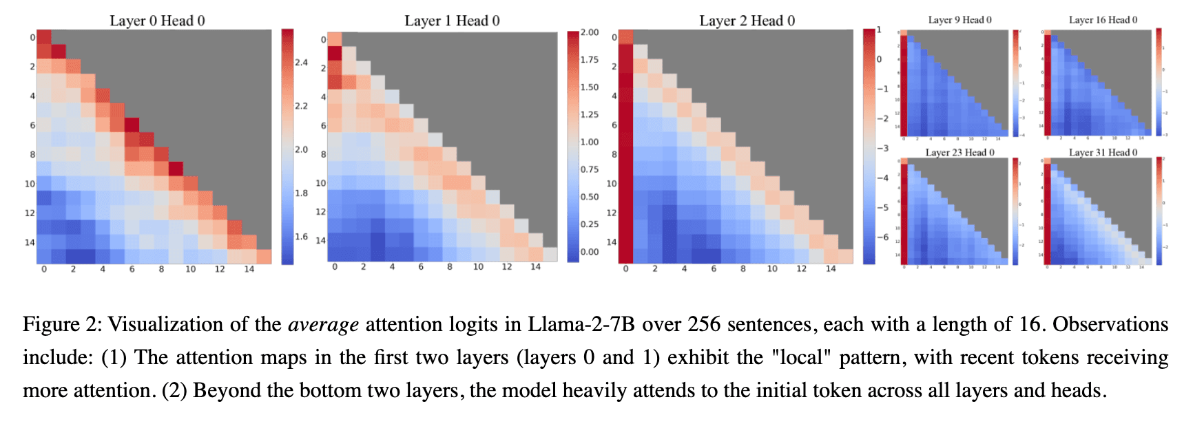
Figure 1: Attention (heat)map from the StreamingLLM paper: A lot of attention is consistently allocated to the first token and to the last neighboring tokens (local attention)
Exploring ways to reduce memory footprint of the KV cache
Let's explore ways to reduce the memory footprint of the KV cache by examining each component of the formula:
Optimizing Batch Size (b)
While decreasing the batch size can indeed alleviate the memory footprint of the KV cache and subsequently reduce latency, it's generally not preferable. This is because reducing the batch size lowers hardware utilization, diminishing cost efficiency. In upcoming posts, we'll delve into why increasing the batch size is often more desirable.
Optimizing Sequence Length (seq_len)
To mitigate the dependency on the total sequence length3, one approach is to refrain from storing keys and values for all tokens in the sequence. This strategy might involve recomputing missing keys and values on each iteration, prioritizing computational resources over GPU memory consumption, especially when memory bandwidth is a limiting factor.
3 Attention Pattern Analysis:
- Strong attention to first tokens
- Local attention clusters
- Special token importance
- Periodic patterns at:
- Sentence boundaries
- Paragraph breaks
- List elements
Another perspective involves not storing keys and values for tokens that the model pays little or no attention to. This could be intentional in models trained to attend only to specific parts of the sequence, such as Mistral-7B, which utilizes sliding window attention (SWA) or local attention. With SWA, attention layers focus solely on neighboring tokens (only 4096), limiting the number of tensor pairs stored per sequence to the window size (4096).
More Methods for Memory Reduction
StreamingLLM Framework
Targeting models with finite-length context windows, this framework observes that initial tokens gather significant attention4. It builds a sliding window by retaining only the first positional tokens ("sink tokens") and the last neighboring tokens (local attention) in the cache. The cache has a fixed length with both a fixed part and a sliding part.
4 StreamingLLM Memory Usage:
Fixed part = n_sink tokens
Sliding part = window_size tokens

Total Memory = (n_sink + window_size) × token_size
vs. Original = full_context × token_size

Typical savings: 40-60% with minimal performance impactH2O and Scissorhands Methods
These methods compress the KV cache by setting a maximum number of cached tokens (budget) and discarding tokens when the cache budget is reached. H2O discards one token at a time, while Scissorhands drops tokens based on a target compression ratio. Both methods exploit the observation that influential tokens at a given step tend to remain influential in future steps.
Cache Eviction Policy - Both H2O and Scissorhands employ cache eviction policies to determine which tokens to discard. Scissorhands retains the most recent tokens and tokens with the highest attention scores within a history window. H2O discards tokens with the lowest cumulated attention scores, retaining tokens consistently achieving high attention scores across iterations.
FastGen Method
FastGen focuses on preserving model accuracy5 by setting a maximum approximation error for the attention matrix instead of a cache budget. It profiles the model's attention layers to determine compression policies during a prefill phase. These policies, such as keeping special tokens or punctuation tokens, are applied to the KV cache at each generation step to meet the error target. If the target is too stringent, FastGen falls back to regular KV caching.
5 FastGen sets an error threshold (ε) for approximation:
Error = ||A - A'||_F / ||A||_F

Where:
A = Original attention matrix
A' = Approximated matrix
||·||_F = Frobenius norm

Typical bounds:
ε = 0.1  → ~70% compression
ε = 0.05 → ~50% compression
ε = 0.01 → ~30% compressionOptimizing Number of Layers (n_layers)
Reducing the number of layers in a language model does not offer significant gains in terms of memory reduction. Typically, smaller models naturally have fewer layers. Therefore, if a smaller model suits your use case and performs adequately, opting for it is a straightforward solution.
Optimizing Number of Attention Heads (n_heads)
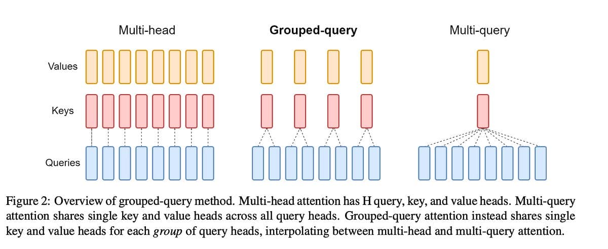
Figure 2: Types of Attention
The multi-query attention (MQA) and grouped-query attention (GQA) architectures provide strategies for reducing the key-value (KV) cache size in models based on the Transformer architecture6. These approaches allow for more efficient use of resources without sacrificing model performance significantly.
6 MQA vs GQA Memory:
MHA: Memory = H × d × 2
MQA: Memory = d × 2
GQA: Memory = g × d × 2

Where:
H = Total heads
d = Head dimension
g = Number of groups (g < H)

Real-world example:
32 heads → 8 groups = 75% reductionIn MQA, all query heads share the same single key and value heads, meaning that each query head computes attention scores using the same keys, and all heads output values computed using the same values but different attention scores.
GQA splits the query heads into groups, with each group sharing the same unique key-value heads. This allows for a smoother reduction in the number of key-value heads compared to MQA, providing a compromise between model representation capacity and KV cache size.
These architectures have been implemented in various models by different research groups, such as Google Research's PaLM, TII's Falcon models, Meta's Llama-2 (limited to 70B only), and Mistral AI's Mistral-7B.
Optimizing Hidden Dimension (d_head)
Once again, there is nothing much to gain here if you are not ready to opt for another model.
Optimizing Precision (p_a)
Quantizing the key-value (KV) cache is an effective method for reducing its size7, but it's important to use quantization algorithms that operate on both weights and activations, not just weights. Algorithms like LLM.int8() or SmoothQuant are suitable for this purpose, as they quantize both weights and activations, resulting in a reduced memory footprint.
7 Precision Impact:
Memory reduction by precision:
FP32 (4 bytes) → FP16 (2 bytes): 50% reduction
FP16 (2 bytes) → INT8 (1 byte): 50% reduction
INT8 (1 byte) → INT4 (0.5 bytes): 50% reductionHowever, for inference tasks, where memory bandwidth is the limiting factor rather than compute power, quantizing the cached tensors before moving them to GPU memory and dequantizing them afterward could suffice. This approach reduces the memory footprint without the overhead of more complex quantization algorithms.
Some inference systems, like FlexGen, NVIDIA TensorRT-LLM, and vLLM framework, already incorporate KV cache quantization features. They store the KV cache and model weights in reduced bit formats (4-bit or 8-bit) dynamically without requiring a calibration step at each iteration.